
Depth Map

A depth map is a heatmap of a picture, which indicates the distance relative to the camera. It contains fundamental 3D information about a picture. In theory a significant portion of a 3D object could be reconstructed just from a picture with a corresponding depth map.
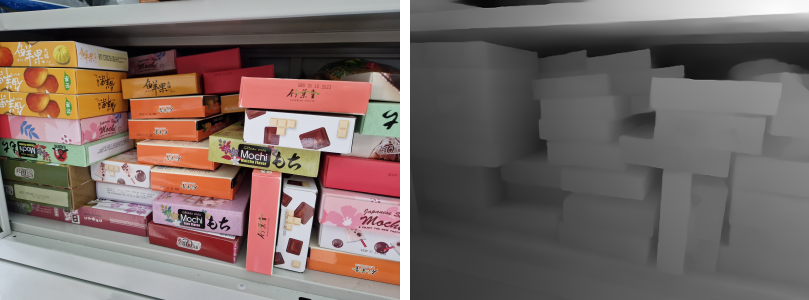
A depth map is typically used for 3D-rendering. There is always a hidden depth channel used for computation purposes. It is required to track what should be drawn. Indeed, when a new object is drawn, for each pixel the depth is compared to the depth on the depth map. Closer pixels are drawn and the depth map is updated. If the pixel is further away, then it is ignored.
There is no universal convention for depth map. For openGL and 3D rendering, the typical convention is 0 (black) meaning close to the camera and 1 (white) meaning far from the camera. However, it can be turned around, and the video game Quake (1996) used both conventions depending on the parity of the frame.
There is also no convention for unit or scale. A depth of 0.5 might mean 1 cm for a picture or 1 km for another. The scale might also not be linear. Only for 3D computation the depth order matters, the scale or unit does not. However for reconstruction it might be required.
MiDaS - depth map from a picture
MiDaS is an AI that computes the depth map of a given picture. Our goal in this post is to give a short explanation of the construction of MiDaS.
Dataset
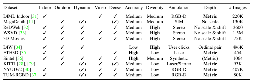
In order to train such a model, a huge dataset with a lot of variety is required. There are not that many datasets. Although some have a lot of pictures, there is often a lack of variety. Various datasets use different way to annotate (LiDAR, hand-annotation, RGB-D camera, stereo camera. Scales are inconsistent, and there is not always a clear way to convert. One of the key ideas of MiDaS is to fuse several datasets and correct the problem with an appropriate loss function.
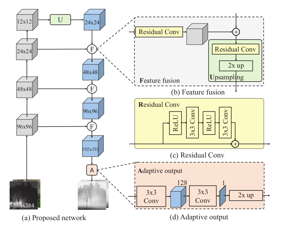
Network architecture
MiDaS is based on a variant of ResNet50
Loss
The disparity space of an image is the pointwise inverse of the depth map. The loss is computed by comparing the disparity spaces. If the 'guessed' disparity space can be rescaled so that it is close to the ground truth disparity space, then the loss is small, on the other hand if no rescaling can match both disparity spaces, then the loss is big.
A second term of the loss is related to discontinuities/derivatives. If the depth map of a picture has some discontinuity, it means that an object ends at this point (we go from a close object to an object in the background, for example). The loss compares the discrete derivative of both disparity spaces.
Training
The network was trained using the Pareto strategy: It is trained on each dataset and the final network is such that any predicion improvement on a dataset reduces the prediction quality on another dataset or datasets.
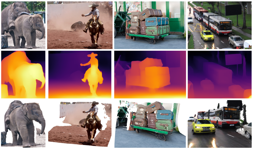
Examples
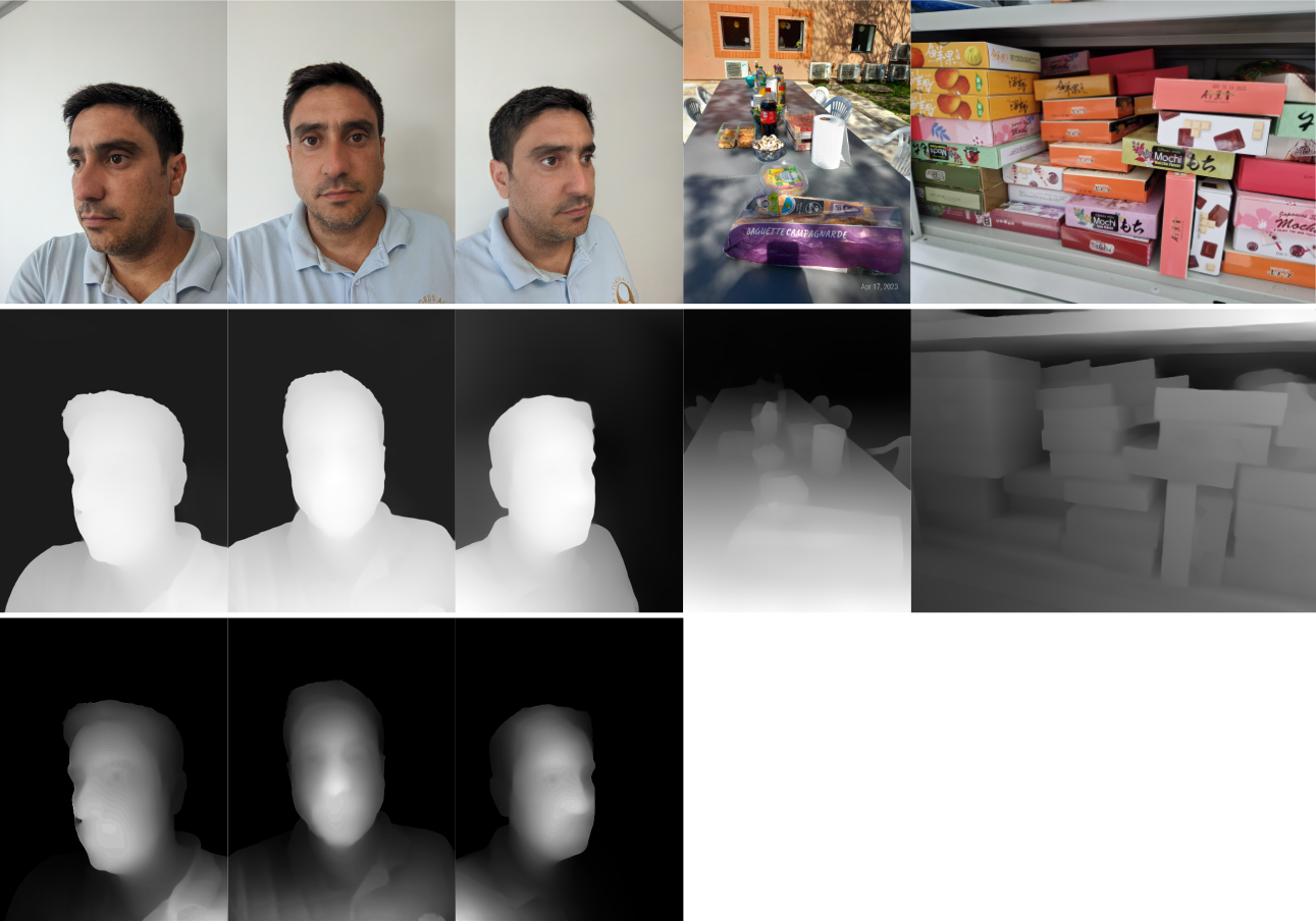
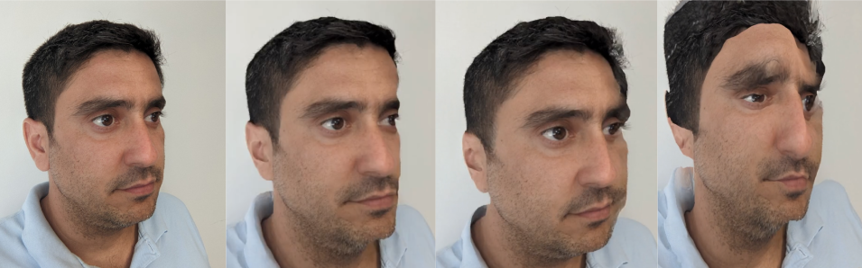
Limits
Once a depth map is computed, one can compute a corresponding 3D model, however the imprecision is too big. If the model is viewed from a different angle, the result is deformed.
Références
- René Ranftl, Katrin Lasinger, David Hafner, Konrad Schindler, and Vladlen Koltun, Towards Robust Monocular Depth Estimation: Mixing Datasets for Zero-shot Cross-dataset Transfer, IEEE Transactions on Pattern Analysis and Machine Intelligence 44, N°3 (2022).
- René Ranftl, Alexey Bochkovskiy, Vladlen Koltun, Vision Transformers for Dense Prediction, 2021 IEEE/CVF International Conference on Computer Vision (ICCV), p.12159-12168.
- Ke Xian, Chunhua Shen, Zhiguo Cao, Hao Lu, Yang Xiao, Ruibo Li, Zhenbo Luo, Monocular Relative Depth Perception with Web Stereo Data Supervision, 2018 IEEE/CVF Conference on Computer Vision and Pattern Recognition, Salt Lake City, UT, USA, 2018, pp. 311-320,
- github DPT